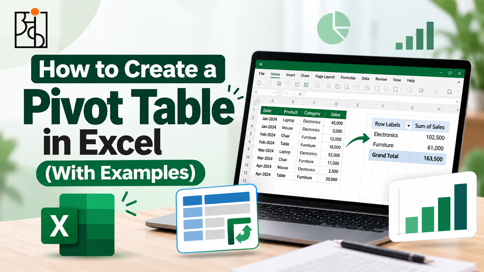
How to Create a Pivot Table in Excel (With Examples)
Almost every Excel user will remember a scenario where they had a few thousand lines of data and knew that there was some information hidden within but had no idea how to find it other than scroll through it. Usually, a pivot table will solve this problem and will change how you interact with your data.
Table of Contents
A pivot table will allow you to take a large, unsorted table of data and summarise it (summing, averaging, counting etc) in exactly the format you want. This guide will show you how to create one from scratch and really help you understand the concept behind them.
What is a Pivot Table?
Before creating a pivot table it is important to understand what they are. As the name suggests it can be a bit of a mystery! Imagine you have sales data in a spreadsheet with a few thousand rows. Each row represents a sale so you will have a date, region, product category, salesperson and revenue column. This gives you no information!
A pivot table allows you to ask a specific question of your data such as what was the total revenue by region or which product category is our best seller each month. This will give you a clean summary of your data in seconds. You won’t have to create any SUMIF functions or manually filter any data. It is called a pivot table because you can ‘pivot’ the data to give you a different summary. This is done by simply moving the fields around.
Example Dataset
Imagine you have a simple sales dataset with the following columns;
Date, Region, Product Category, Salesperson, Units Sold, Revenue.
You have a few thousand rows of data and this represents a years worth of sales across 4 regions and 3 product categories. This would be very hard to read in its raw format however by pivoting the data it becomes very useful.
Read More: Why Data Analytics Projects Matter So Much for Beginners
Step 1 – Ensure data is clean

This is a common mistake. If your data is not clean then your pivot table will not be clean. Firstly ensure that all your columns have headers, no blank rows and your date columns are actual dates.
If there is one blank row in your data then Excel will only pull data from above this row. This can be a small issue however it is a very common error. Have a quick look through your data to ensure there are no blank rows.
Step 2 – Select your data and insert a pivot table

Once your data is clean click anywhere within your data. Excel should automatically detect the correct range. Then go to Insert → PivotTable. Excel will now open a new window. Confirm that the range has been detected correctly and choose where you want your pivot table to go. Usually a new worksheet will be best.
Click OK. A blank pivot table will appear. On the right-hand side of your screen you will now have a PivotTable Fields box containing all of your columns.
Read More: How to Think Like a Data Analyst (Even If You’ve Never Touched a Spreadsheet
Step 3 – Create your first summary

This is where it really starts to look magical! There are 4 boxes within the PivotTable Fields box;
Filters, Columns, Rows, Values.
All you need to do within a pivot table is move your fields into these boxes.
To create your first summary drag the Region field into the Rows box and the Revenue field into the Values box. Your pivot table will now show you the total revenue for each region. This will take you hours to do manually however can be done in around 4 seconds!
Now drag the Product Category field into the Columns box. The pivot table will now reorganize itself to show you a cross tab. This will show you the revenue by region and by product category. This is usually where you realise how much quicker this is than manually.
Read More : Online vs Offline Data Analytics Course Which Is Actually Better?
Step 4 – Change what is being calculated

By default if you drag a numerical field into the Values box it will calculate it using a SUM function. However you may not want this to happen. To change this click on the small arrow next to your field in the Values box. Select Value Field Settings. A list of calculations will now appear;
Average, Count, Max, Min etc.
Changing this to an Average function will instantly show you the average revenue per transaction. This is the same layout however you can gain different insights. This is where a huge amount of the real power comes in. The same table can provide you with different answers.
Step 5 – Filtering

Dragging the Date field into the Filters box will give you a drop down box at the top of your table. This will allow you to view all of your data or filter it to a specific month/quarter. This is actually very useful!
To make it more visual go to Insert -> Slicer. This will allow you to create buttons for a field like Region or Salesperson. This will mean you don’t have to go through a drop down menu. Slicers can be very useful if you want to share your pivot table with someone who doesn’t want to deal with the interface. It will make your table behave more like an interactive dashboard.
Step 6 – Formatting

A very basic pivot table can look very cluttered. Right click on your table and go to PivotTable Options (or use the style options from the Design tab). This will allow you to quickly clean up your pivot table. This will include adding banded rows, clearer borders and formatting your numbers (currency symbols, thousand separators etc).
Rename your default Sum of Revenue heading to Total Revenue. This will make your pivot table easier to understand. The default headings provided by Excel are very functional however are not ideal if you want to create a report.
Example – Find the poor performing region

Putting it all together, let’s take a look at how it would appear in practice. Using your sales data drag the Region field into the Rows box and Revenue into the Values box. This will instantly tell you the total revenue per region. Now add the Product Category field into the Columns box. This will now tell you the revenue per region and per product category. This may tell you that one region is performing okay however all of their revenue is coming from one product category and others are performing very poorly.
Now add the Date field into the Filters box. Now you can filter this to only show you data from the most recent quarter. This could show you that a region that appeared very strong throughout the year is actually declining in the last few months. This is the real power of pivot tables. They help you ask multiple questions of your data in minutes.
Common Errors
There are a few common errors when starting off with pivot tables. Firstly forgetting to refresh your pivot table when the data changes. When new data is added to the source data your pivot table will not automatically refresh. Right click on your table and select Refresh.
Another common error is placing your fields in the wrong boxes. If you have a numerical field (such as Revenue) and place it in the Rows box you will get a very confusing list of all the unique values of your revenue. This does not mean it is broken however it is due to the field being placed in the wrong box.
The most common reason for a pivot table appearing to be incorrect is because the data is not clean (as mentioned above). This is simply a correct summary of your dirty data.
Why it is an Important Skill to Learn
Pivot tables can easily be seen as a tool specific skill (useful but not much more than they know Excel). However the real skill being developed is taking a mass of raw data and changing the format so it can answer the question you want. This is a very practical skill.
This is exactly what Ankashram focuses on heavily when teaching data analytics. We want you to get used to taking raw data and turning it into something that can be used to make a decision. Often pivot tables are the starting point of this as you can see instant feedback from moving your fields.
Get Used to Pivot Tables Faster
The best way to get good at this is to open up a real dataset and play around with moving your fields. Try moving the same field into a different box. Try changing your calculation from a Sum to an Average or Count. This will help you get used to pivot tables.
This is a big part of how Ankashram delivers practical training. We use a real dataset that is not completely clean. This is where the skill will really stick. Creating a pivot table from a perfectly clean practice file will not teach you as much as one that contains a blank row, inconsistent dates and some random duplicates.
Frequently Asked Questions
Q1. Do I need to know advanced Excel to create a pivot table?
No! Pivot tables are designed to help you summarize your data without using any formulas. Simply drag your fields into the correct boxes within the Rows, Columns and Values sections. Most people can create a useful pivot table within minutes.
Q2. My pivot table is not updating when I add new data
Pivot tables will not automatically update when the source data changes. Right click anywhere on your pivot table and select Refresh. Or go to Data → Refresh All.
Q3. Can I use pivot tables with large amounts of data?
Yes! Pivot tables are specifically designed for this. They can usually cope with tens of thousands of rows. If you have a very large amount of data you can improve the performance by importing into Excel’s Power Pivot or Power Query.
Q4. What is the difference between a pivot table and a table with formulas?
A table with formulas such as SUMIF will require you to recreate or amend your formulas. Whereas with a pivot table you can simply move your fields around to give you a completely different summary.
Q5. Why am I getting a list of numbers?
Most likely you have moved a numerical field into the Rows or Columns section. Move it into the Values section. Excel will automatically apply a calculation such as a Sum or Average.
Q6. How will learning pivot tables help me with data analytics?
Pivot tables teach you the key habit of most data analysis. Taking raw data and changing the format to answer your question. We see this as an essential practical skill. The same instinct will be used in more advanced tools and techniques.