How to Remove Duplicates in Excel
Duplicate entries are a very common occurrence in spreadsheets. They are there while combining files, importing data, or simply when you are just using your “Ctrl + C and Ctrl + V”. If you find duplicates remaining in the sheet, they will give you the wrong readings for totals, averages, and ultimately wrong conclusions.
Table of Contents
If your target is to remove all the duplicates, and retain the unique records at the same time, here’s how to do it!
Why duplicates can be an issue:
Duplicates lead to:
Doubled values (revenue/quantities)
Appearances of having more values than you actually have.
Multiple problems when you are making Pivot Tables or Power BI
Confusion while comparing different records.
Filtering out the duplicates doesn’t just help you but also makes sure that everything is of the right quality.
Golden Rule
Always maintain a copy of the data.
Right click the sheet tab, select copy, and mark the ‘create a copy’ option and then work on that copy. Don’t edit the original until you have properly finished the data.
Method 1 – Eradicate Duplicates.
This method works best when the number of duplicates is known.
Click on any cell in your tab of the sheet.
Go to the Data tab.
Click the Remove Duplicates option.
Tick the columns which will be used to determine if two rows are duplicates.
Mark the columns that will be used in order to determine if two rows are duplicates.
Select Ok.
Excel will display the number of duplicates it has removed and how many remaining unique values are there.
In the end, just mark the columns that are supposed to be used to determine if a record is unique. For instance, Order, Email. If you mark all of your columns Excel will only delete the rows that are replicas of each other.
Read More: How to Think Like a Data Analyst (Even If You’ve Never Touched a Spreadsheet
Method 2 – Highlight Duplicates.
This is a method if your main task is to find out where exactly the duplicates are.
Highlight the column(s).
The procedure after this is,
Go to Home
Conditional Formatting
Highlight Cells Rules
Duplicate Values.
Select the way you would like to highlight the duplicates and select OK.
Your duplicates will now be highlighted. You can then filter out by colour, and then manually check them. This is useful if there are records that have the same values.
Read More: Why Data Analytics Projects Matter So Much for Beginners
Method 3 – Advanced Filter.
The use of this method is; Producing a set of clean data, comprising your own records.
Highlight your data.
Go to Data
Click on Advanced (Sort & Filter)
Select ‘Copy to another location’.
Mark,‘records only’.
Select a cell for your data to go to.
Check OK.
You are now with a range with the unique records only. If you are satisfied with the records, you can move ahead and the replacement of the original data can take place.
Method 4 – Power Query ( for large and recurring data)
This method provides you with the control and also helps create a log of everything you have done.
Highlight your data.
Go to Data
From Table/Range.
In the Power Query Editor select your columns from the tab.
Go to Home
Select Remove Rows
Then, Select Remove Duplicates.
Click on Close & Load.
You are now provided with a sheet of cleaned data. There is also a log so that you can refresh the query at a date if you’ve got new data. That is useful if you regularly clean that type of file.
This further helps in Avoiding losing any records.
Decide which of the columns will be used which will help to determine if the record is unique. You will probably end up with a unique column or a combination of columns.
Don’t just tick all your columns.
If you have two columns and both of them have different important information, then don’t remove the duplicates.
After the duplicates have been removed, check the totals to make sure they haven’t been affected significantly. If they have, then you need to find out why.
Make a copy of your original until you’re completely done.
Example
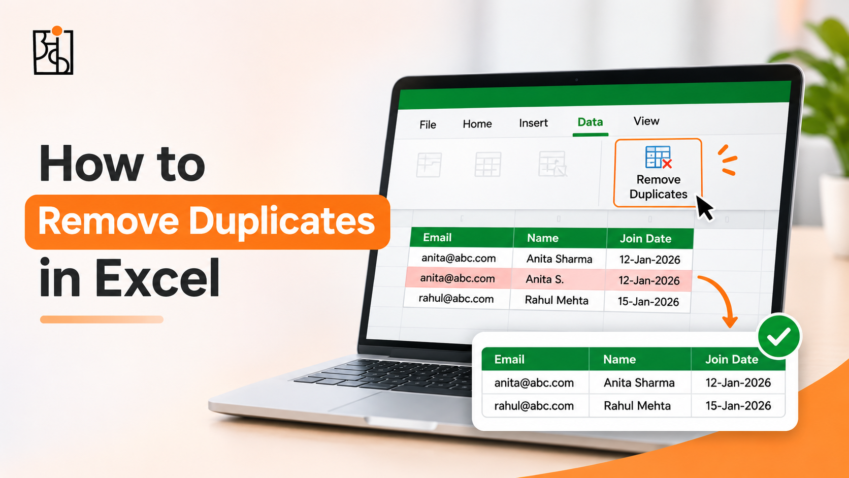
Let us think that we have a customer list with multiple columns: Email, Name and Join Date.
Two of the records have the same email address but slightly different names (typos). Now as our unique column is email we can remove the duplicates on the basis of that column.
If we’d selected all columns then Excel would have left both records as they have (they have names).
Useful Tips
Use the TRIM function or the Power Query options to remove any spaces.
Turn your range into an Excel Table
Make a note of the columns being used to find duplicates
Ankashram is all about data programmes, Think with Data being one of them. Clean data is absolutely fundamental to analysis and one of the ways of achieving clean data is to get rid of duplicates.
Frequently Asked Questions
Q1.Will it retain the last record?
Excel will keep the instance of the record and delete the others. If you want a record then sort the Excel data first so that the record you want is at the top.
Q2. Can I undo?
Yes you can undo immediately by pressing Ctrl. Z. Once you’ve saved and closed it though it becomes a lot harder to undo. That’s why it’s so important to use a copy.
Q3.What if they’re not exact duplicates?
If the duplicates have only minor differences in spelling, spacing or capitalisation then Excel won’t pick them up with the standard tool. Use the TRIM/CLEAN functions or the fuzzy options in Power Query. Just manually check the highlighted rows.
Q4.Is Power Query better than the button?
If it’s a one off then the standard tool is fine. If you’re doing it regularly or have files then Power Query is the better and more consistent choice.
Q5.How does Ankashram teach data cleaning?
Ankashram is all about habits to keep the data clean. Ankashram will make sure that you remove the duplicates properly and thoroughly.