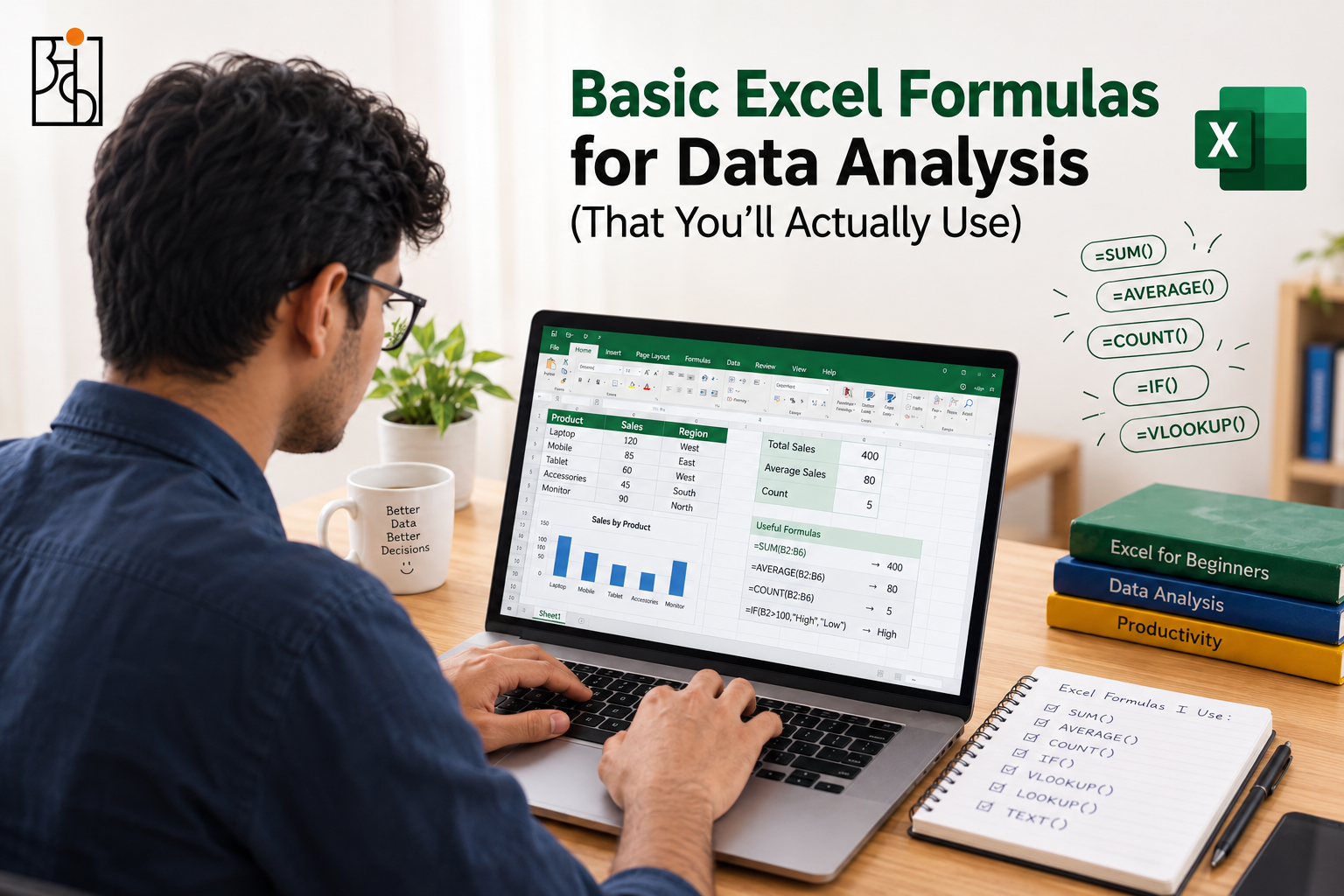
Basic Excel Formulas for Data Analysis (That You’ll Actually Use)

Excel formulas for data analysis are what separate someone who just types numbers into a grid from someone who can actually answer a manager’s question in minutes. Rohan learned this the hard way. He inherited a sales spreadsheet with fourteen months of transactions, no summary tab, and a manager who wanted to know “how we’re doing by region” by end of day. He spent the first hour doing exactly what most people do in that situation — manually filtering, copying numbers into a separate sheet, adding them up by hand, and hoping he hadn’t missed a row. A colleague glanced over his shoulder, typed a single SUMIFS formula, and had the entire regional breakdown done in under a minute. Rohan wasn’t bad at his job. He just didn’t know the formulas that make Excel actually useful for this kind of work, rather than just a grid for typing numbers into.

That gap — between using Excel as a glorified table and using it as a genuine analysis tool — comes down to a fairly small set of spreadsheet formulas that cover the overwhelming majority of real analytical work. None of them require a statistics background or a coding class. They just need to actually be learned once, properly, rather than half-remembered from a tutorial watched years ago.

Excel Formulas for Data Analysis: Quick Reference Table

Formula	Syntax / Example	What It Does
SUM	=SUM(C:C)	Adds up a range of numbers
SUMIF	=SUMIF(B:B, "North", C:C)	Adds values in a range only where one condition is met
SUMIFS	=SUMIFS(C:C, B:B, "North", D:D, "January")	Adds values where multiple conditions are met
COUNTIF	=COUNTIF(A:A, "Pending")	Counts how many cells meet one condition
COUNTIFS	=COUNTIFS(A:A, "Pending", B:B, "North")	Counts cells meeting multiple conditions
AVERAGEIF	=AVERAGEIF(B:B, "North", C:C)	Averages values that meet one condition
AVERAGEIFS	=AVERAGEIFS(C:C, B:B, "North", D:D, "January")	Averages values meeting multiple conditions
VLOOKUP	=VLOOKUP(A2, ProductTable, 3, FALSE)	Looks up a value and returns a related value from a column to its right
XLOOKUP	=XLOOKUP(A2, ProductTable[ID], ProductTable[Name])	Modern lookup that works left or right and handles missing matches better
INDEX + MATCH	=INDEX(C:C, MATCH("North", B:B, 0))	Flexible lookup that can work in any direction
IF	=IF(C2>1000, "High Value", "Standard")	Returns one value if a condition is true and another if false
Nested IF	=IF(C2>5000, "High", IF(C2>1000, "Medium", "Low"))	Handles more than two categories using multiple IF conditions
IFS	=IFS(C2>5000, "High", C2>1000, "Medium", TRUE, "Low")	A cleaner alternative to nested IF for multiple categories
IFERROR	=IFERROR(VLOOKUP(A2, ProductTable, 3, FALSE), "Not Found")	Replaces an error result with a custom message
TRIM	=TRIM(A2)	Removes extra, leading, and trailing spaces from text
CONCATENATE / &	=A2&" "&B2	Joins text from multiple cells
TEXTJ	=TEXTJOIN(", ", TRUE, A2:D2)	Joins multiple cells with a separator while skipping blank cells

SUM, SUMIF, and SUMIFS: The Foundation of Almost Everything

SUM itself barely needs an introduction — it adds up a range of numbers. The real value starts with SUMIF, which adds up a range only where a condition is met. =SUMIF(B:B, “North”, C:C) adds every value in column C where the matching cell in column B says “North,” which is exactly the kind of question — “how much did we sell in this specific region” — that comes up constantly in real analysis.

SUMIFS extends this further by allowing multiple conditions at once, which is where it becomes genuinely powerful. =SUMIFS(C:C, B:B, “North”, D:D, “January”) adds sales only where the region is North and the month is January, letting a single formula answer a question that would otherwise take several manual filtering steps to work through. Rohan’s colleague used exactly this structure to produce a full regional breakdown in one pass instead of filtering the sheet four separate times.

COUNTIF and COUNTIFS: Answering “How Many,” Not “How Much”

Where the SUM family totals values, the COUNT family counts occurrences, and the distinction matters more than it sounds like it should. =COUNTIF(A:A, “Pending”) answers “how many orders are still pending,” a question SUM can’t touch since there’s no number to add, only a status to tally.

COUNTIFS works the same way SUMIFS does, layering multiple conditions into one count. =COUNTIFS(A:A, “Pending”, B:B, “North”) narrows that same question down to pending orders specifically in the North region. This combination shows up constantly in quality checks too — counting how many rows have a blank value in a required column, or how many entries fall outside an expected range, both of which flag data problems before they quietly distort a larger analysis.

AVERAGEIF and AVERAGEIFS: Because a Total Alone Can Mislead

A sum tells you the total. It says nothing about whether that total came from five enormous orders or five hundred small ones, and that distinction changes what a number actually means. =AVERAGEIF(B:B, “North”, C:C) returns the average order value for the North region specifically, filling in exactly the gap a plain SUM leaves open.

AVERAGEIFS layers on additional conditions the same way its SUM and COUNT cousins do. Used together, SUM, COUNT, and AVERAGE for the same slice of data — total sales, number of orders, average order value — tend to tell a far more complete story than any single one of the three would on its own, since a change in the total can be driven by more orders, bigger orders, or some mix of both, and only looking at all three at once actually reveals which.

Read More:  How to Make Data-Driven Decisions Without Getting Lost in the Data

VLOOKUP and XLOOKUP: Pulling Information From Somewhere Else

Real analysis rarely lives in one tidy table. A sales sheet might list a product ID, while the actual product name and category sit in a completely separate reference sheet, and connecting the two by hand, row by row, is exactly the kind of tedious work a lookup formula exists to eliminate.

VLOOKUP handles this by searching for a value in the first column of a range and returning a corresponding value from a specified column to its right: =VLOOKUP(A2, ProductTable, 3, FALSE) looks up the product ID in A2 within the ProductTable range and returns whatever sits in the third column of that table — the product name, say. The FALSE at the end matters more than it looks like it should, since it forces an exact match rather than an approximate one, and an approximate match on something like a product ID can quietly return completely the wrong row.

XLOOKUP, available in newer versions of Excel and in Google Sheets, does the same job with fewer of VLOOKUP’s rough edges — it can look left as well as right, doesn’t break as easily when a column gets inserted into the source table, and handles a missing match more gracefully. =XLOOKUP(A2, ProductTable[ID], ProductTable[Name]) reads almost like plain English once the syntax clicks, and it’s worth learning directly if the software available supports it, rather than defaulting to VLOOKUP purely out of habit.

Read More: How to Improve Logical Thinking: A Practical Guide to Thinking Critically

INDEX and MATCH: The More Flexible Alternative

INDEX and MATCH, used together, solve the same basic problem as VLOOKUP but with more flexibility, which matters once a dataset gets more complicated than a simple left-to-right lookup. MATCH finds the position of a value within a range — =MATCH(“North”, B:B, 0) returns which row contains “North” — and INDEX then returns a value from a specific position within another range. Combined, =INDEX(C:C, MATCH(“North”, B:B, 0)) returns the value in column C that sits on the same row where “North” was found in column B.

The real advantage over VLOOKUP shows up when the lookup column isn’t conveniently positioned to the left of the answer, a situation VLOOKUP genuinely can’t handle without rearranging the data first. INDEX and MATCH don’t care which direction the answer sits in relative to the search column, which makes this combination considerably more durable as a spreadsheet grows and changes shape over time.

IF, Nested IF, and IFS: Building Logic Into a Sheet

IF is the formula most people learn first and use the least effectively. =IF(C2>1000, “High Value”, “Standard”) labels an order based on whether it crosses a threshold, and that simple structure is the building block for a huge share of the categorization work that shows up in real analysis — flagging outliers, grouping continuous numbers into buckets, marking records that need a closer look.

Nesting multiple IF statements inside each other handles more than two categories, though it gets messy and hard to read fast: =IF(C2>5000, “High”, IF(C2>1000, “Medium”, “Low”)) works, but a fourth or fifth category makes a nested IF formula genuinely difficult to debug later. IFS solves this cleanly in newer Excel versions: =IFS(C2>5000, “High”, C2>1000, “Medium”, TRUE, “Low”) reads each condition in order and stops at the first one that’s true, without the nested parentheses piling up.

Read More: How to Think Like a Data Analyst (Even If You’ve Never Touched a Spreadsheet

IFERROR: Catching Problems Before They Spread

A single broken lookup or a division by zero can quietly turn one wrong number into dozens of wrong numbers if other formulas reference the broken cell. =IFERROR(VLOOKUP(A2, ProductTable, 3, FALSE), “Not Found”) catches exactly this — if the lookup fails for any reason, the cell displays “Not Found” instead of an ugly #N/A error that a formula built on top of it would otherwise inherit silently.

This matters more than it sounds like it should in any sheet built for repeated use rather than a one-off analysis. A dashboard that updates automatically as new data comes in will eventually hit a row with a genuinely missing reference, and wrapping the risky formulas in IFERROR means that one bad row produces a clear, visible flag rather than a cascade of broken calculations spreading quietly through the rest of the sheet.

Read More : Comic by Ankashram – Ask Tough Questions with Your Data Analyst

TRIM, CONCATENATE, and TEXTJOIN: Cleaning Up Messy Text

Real data is full of small text problems that break formulas relying on exact matches — an extra space at the end of a name, inconsistent capitalization, a city name that appears three different ways because three different people typed it in over the years. TRIM removes leading and trailing spaces along with extra spaces between words, which alone fixes a surprising share of lookup failures that actually trace back to invisible whitespace rather than any real data problem.

CONCATENATE (or the simpler & operator) joins text together — =A2&” “&B2 combines a first and last name into one cell — which comes up constantly when building a unique identifier out of several separate fields. TEXTJOIN improves on this for joining multiple cells at once with a consistent separator, without needing an & between every single piece: =TEXTJOIN(“, “, TRUE, A2:D2) joins everything in that range with a comma and space between each value, skipping any blank cells along the way.

Read More : How to Get a Data Analyst Job: What Actually Moves the Needle

Putting a Few of These Together

The real value of these formulas rarely shows up one at a time. Rohan’s actual regional breakdown, once he learned the pattern, combined several of them: SUMIFS for total sales by region, COUNTIFS for order volume in that same region, AVERAGEIFS to catch whether the total was being skewed by a handful of unusually large orders, and IFERROR wrapped around the whole thing so a missing region label didn’t break the summary entirely. None of those four formulas is complicated on its own. Combined, they turned a task that used to take an anxious hour of manual filtering into something that updates instantly every time the underlying data changes.

Why Learning the Formula Beats Memorizing the Answer

It’s tempting to just search for “how do I get a regional sales total in Excel” and copy whatever formula shows up, and that works fine for a one-off task. It falls apart the moment the question changes slightly — a manager who wants the same breakdown by product category instead of region, or by month instead of both. Understanding what SUMIFS is actually doing, rather than just pattern-matching a specific formula to a specific question, means adapting it to the next slightly different question takes thirty seconds instead of another search and another copy-paste.

This is really the whole case for learning these spreadsheet formulas properly rather than treating Excel as a tool to look things up in as needed. The underlying logic — filter by a condition, then sum, count, or average what’s left; look up a related value from somewhere else; build a category based on a threshold — repeats constantly across genuinely different business questions. Learn the pattern once, and most of what looks like a new problem turns out to be the same handful of formulas applied to a slightly different column.

Frequently Asked Questions

Q1.Do I need to learn all of these formulas, or just a few?

SUMIFS, COUNTIFS, and either VLOOKUP or XLOOKUP cover a large share of everyday analytical work on their own. The rest are genuinely useful, but those three are the ones worth learning first and learning well.

Q2.What’s the real difference between VLOOKUP and INDEX/MATCH if they do the same thing?

VLOOKUP is simpler to write but requires the lookup column to sit to the left of the answer column, and it can break if columns get rearranged later. INDEX and MATCH handle lookups in either direction and tend to hold up better as a spreadsheet evolves, at the cost of being slightly more complex to write the first time.

Q3.Should I switch to XLOOKUP if my version of Excel supports it?

Generally yes — XLOOKUP handles most of VLOOKUP’s common failure points more gracefully and reads more intuitively once you’re used to the syntax. The main reason to stick with VLOOKUP is compatibility with older files or software that doesn’t support the newer function yet.

Q4.Why does my formula show a #N/A or #DIV/0! error even though the data looks fine?

Usually an invisible text issue — extra spaces, a mismatched data type, or a genuinely missing match. Wrapping the formula in IFERROR won’t fix the underlying data problem, but it stops that one error from breaking other formulas that reference the same cell, and it’s often the fastest way to spot which specific rows actually need a closer look.